Why you might be fitting Arrhenius data badly

The Arrhenius equation describes the behaviour of a rate constant, \(k_r\), as a function of temperature, \(T\),

\[k_r = A \exp{\bigg(\frac{-E_a}{RT}\bigg)},\]

where \(E_a\) is the activation energy, \(R\) is the ideal gas constant, and \(A\) is a pre-exponential scaling factor. The Arrhenius equation is used widely in the chemical sciences and features prominently in early undergraduate courses and textbooks¹. The Arrhenius equation can be used to describe the relationship between measured rate constants as a function of temperature and therefore provide estimates of activation energy and pre-exponential factor (the Arrhenius parameters). However, despite being more than 130 years old, the Arrhenius equation is still used in a way that distorts the estimates of these parameters.

In particular, the problem comes from the “linearisation” of the Arrhenius equation. This is where the exponential problem above is manipulated to give a linear problem with the form

\[\ln{(k_r)} = -\frac{E_a}{R}\frac{1}{T} + \ln{(A)}.\]

And by plotting the natural logarithm of the rate constant against the reciprocal temperature, we can fit a straight line with gradient \(-E_a/R\) and intercept \(\ln{(A)}\). The convenient reformulation is great for use in the classroom, where drawing a straight line through points is much easier than fitting an exponential relationship. But it should not be used in formal analysis in academic publications (yet, it is regularly – I won’t shame anyone in particular though).

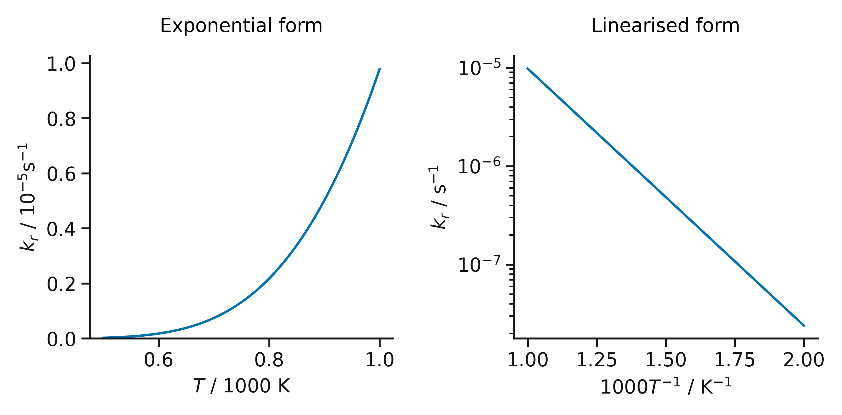
The effect of linearization of the Arrhenius equation.

Before we dive into why using the linearised Arrhenius equation is so problematic for data analysis there are some important aspects of uncertainties and data modelling to consider.

1. Generally speaking, the uncertainty in the measurement of a rate constant will be normally distributed.

Let’s think about the rate constant for some reaction. For a given temperature the true rate constant is single-valued, there is only one value that quantifies the rate and direction of our chemical reaction. However, when we measure the rate constant some (random and systematic) uncertainty is introduced. Even with a perfect measurement device (where there is no systematic uncertainty), there will always random uncertainties which we cannot control. These random uncertainties sum in the measurement of our physical quantity, meaning that repeated measurements of our rate constant will result in a normal distribution of values, centred on the true rate constant with some variance².

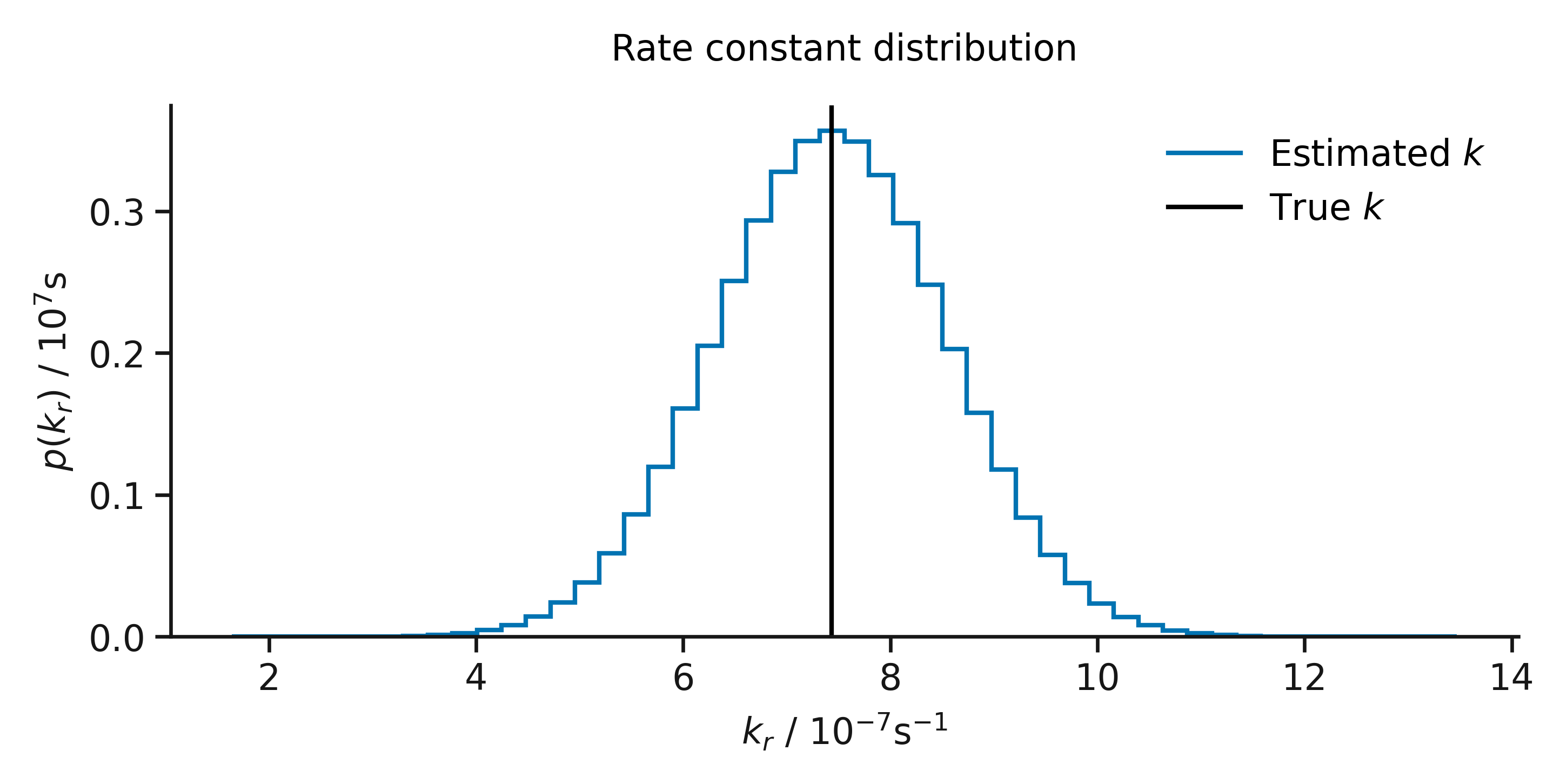
A normally distributed rate constant.

2. Most least squares assume normally distributed data.

Least squares is a mathematical process to find model parameters; i,e. the coefficients of a polynomial that describes our data. We can see how linear least squares works in the video below, where the difference between the model (the straight line) and the data (the holes) is minimised to give the “line of best fit”³. An assumption of most least squares methods is that the data are drawn from a normally distributed parameter, which we can see in the maximum likelihood approach to ordinary least squares.

In linear regression, the observations (dots) are assumed to be the result of random deviations (strings) from an underlying relationship (stick). A simple but highly visual practical implementation of the "line of best fit" [more: https://t.co/ASnVxNMevD]pic.twitter.com/FI4BeXmbiG

— Massimo (@Rainmaker1973) April 19, 2023

So why does this mean that using a linearised Arrhenius form is problematic? When we take the logarithm of the rate constant, we take the logarithm of a normally distributed variable – it is no longer normally distributed. This means that in using the linear Arrhenius form, we ignore the assumptions of the ordinary least squares that we then use to estimate the activation energy and preexponential factor.

The effect of ignoring this assumption is that we bias the result of our fitting. Below, the result of performing linear and non-linear fitting on the two forms of the Arrhenius equation are shown. This is from fitting 2¹⁴ data sets, where the values of the rate constant were drawn from normal distributions. It is clear that by using the linear form of the Arrhenius equation we significantly bias the result that we observed, we are much more likely to underestimate the activation energy.

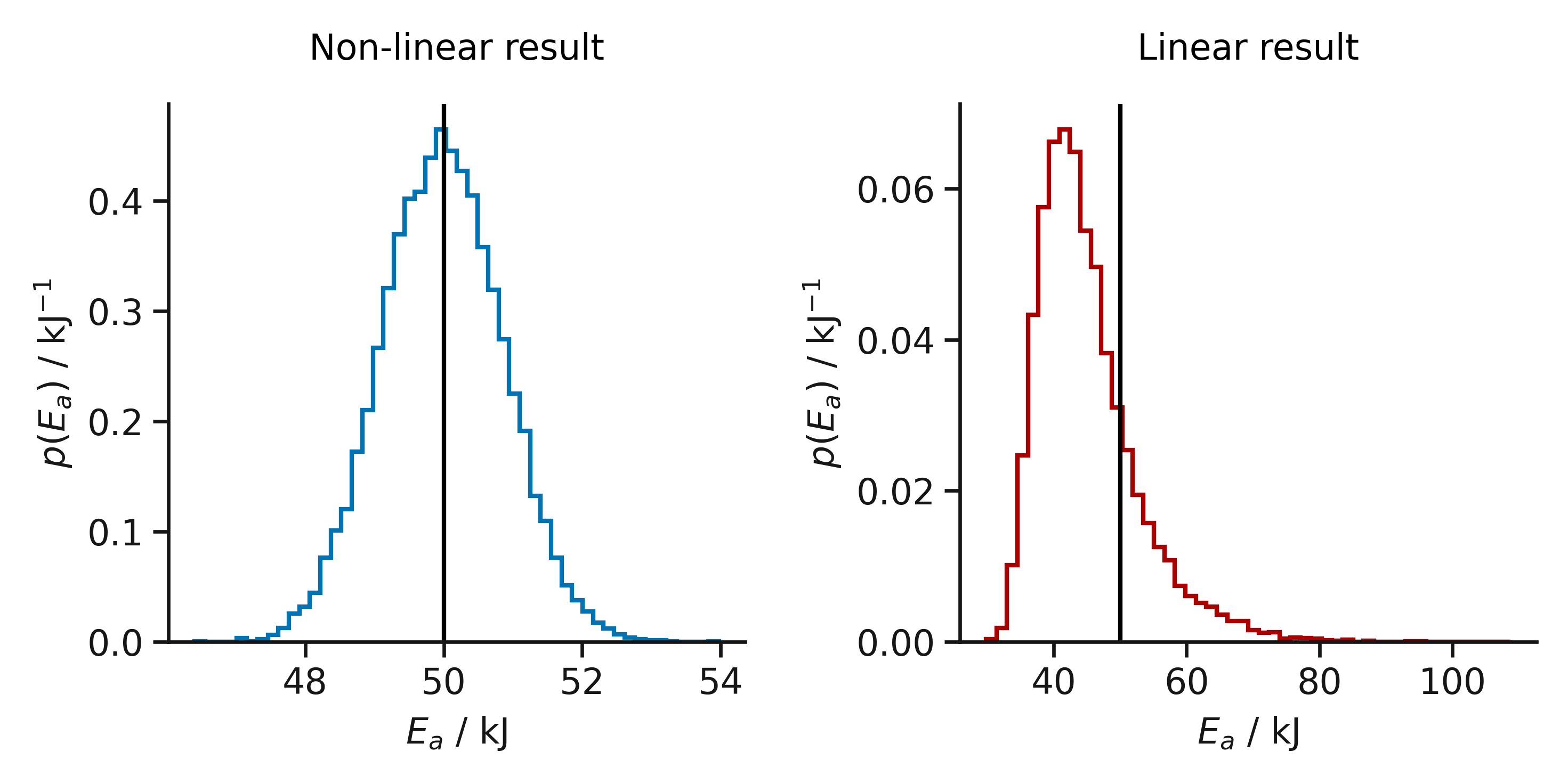
The bias introduced in using linear least squares for Arrhenius behaviour, the vertical line represents the true activation energy.

While there is important historical and pedagogical context to the linearisation of the Arrhenius equation, it is not acceptable to introduce such clear bias to the results of formal scientific analysis. I hope that this blog will make others think more carefully about the analysis that they perform and, if they don’t already, they will start to fit Arrhenius data using the non-linear approach. To aid this, I have included some Jupyter Notebooks that enable ordinary and weighted non-linear regression to be performed⁴.

1. For example, there is a section on it in Atkins’ Physical Chemistry (pages 799-803 in the ninth edition). ↩

2. Indeed, we have shown this to be true for diffusion from atomistic simulation. ↩

3. I have discussed linear least squares previously, mentioning in passing the use of a multi-dimensional normal distribution. ↩

4. Also available as an Excel workbook, but I advise on using the Notebooks. ↩

« previous next »