import pandas as pd
import matplotlib.pyplot as plt
from sklearn.ensemble import RandomForestClassifier
from sklearn.model_selection import train_test_split
from sklearn.metrics import plot_confusion_matrix
Material classification
Neutron scattering can give complementary information about materials, such as the structural information from diffraction and electronic information from spectroscopy. In this exercise, we will look at using a random forest classification of structural and electronic information to create a model that can guess the space group for new materials.
The first thing that we need is some data, I have obtained data for lithium, sodium, and potassium containing materials of the four most common space groups (space group numbers: 2, 14, 15, 19).
This data can be found in the file materials_data.csv.
data = pd.read_csv('materials_data.csv')
This data is read in as a pandas.DataFrame so it can be visualised as so.
data
| pretty_formula | spacegroup.number | band_gap | density | volume | formation_energy_per_atom | nsites | |
|---|---|---|---|---|---|---|---|
| 0 | KAl9O14 | 14 | 4.1426 | 3.142646 | 534.648960 | -3.364229 | 48 |
| 1 | K2Se2O | 15 | 0.0975 | 3.303683 | 253.443517 | -0.940536 | 10 |
| 2 | K2AgF4 | 14 | 0.6151 | 3.343987 | 260.263084 | -2.371859 | 14 |
| 3 | Na2TeS3 | 14 | 1.7919 | 2.904619 | 616.908734 | -1.000993 | 24 |
| 4 | K3Zn2Cl7 | 2 | 3.9024 | 2.345705 | 702.644832 | -1.909423 | 24 |
| ... | ... | ... | ... | ... | ... | ... | ... |
| 537 | Na2Cr2O7 | 2 | 2.5253 | 2.654095 | 655.601817 | -1.869509 | 44 |
| 538 | K4SnO4 | 2 | 2.3423 | 2.977324 | 378.252471 | -1.839865 | 18 |
| 539 | LiTa3O8 | 15 | 3.3841 | 7.889695 | 285.303789 | -3.263699 | 24 |
| 540 | LiSmO2 | 14 | 3.7655 | 6.485182 | 193.881819 | -3.185751 | 16 |
| 541 | K4UO5 | 2 | 2.1910 | 4.207670 | 374.454975 | -2.645721 | 20 |
542 rows × 7 columns
The first thing to do is separate our data into training and validation data (this process is common in machine learning methods).
For this we will use the scikit-learn function train_test_split.
train, validate = train_test_split(data, test_size=0.2)
We have split the data, which consisted of data about 542 materials, so that 80 % will be used to train and the remaining 20 % is reserved for validation.
train
| pretty_formula | spacegroup.number | band_gap | density | volume | formation_energy_per_atom | nsites | |
|---|---|---|---|---|---|---|---|
| 244 | NaInI4 | 14 | 2.4484 | 3.715767 | 1153.737028 | -0.785825 | 24 |
| 205 | Li2SnS3 | 15 | 1.4195 | 3.435021 | 442.395841 | -1.213020 | 24 |
| 99 | Na3DyCl6 | 14 | 5.4269 | 2.831208 | 521.042810 | -2.353868 | 20 |
| 378 | KC2N3 | 14 | 4.5026 | 1.611816 | 433.272097 | -0.278986 | 24 |
| 33 | K5SnBi3 | 14 | 0.0145 | 4.095423 | 1526.391127 | -0.349438 | 36 |
| ... | ... | ... | ... | ... | ... | ... | ... |
| 533 | Na2SnSe3 | 14 | 1.3283 | 3.803238 | 701.320138 | -0.774873 | 24 |
| 303 | K4SiO4 | 14 | 3.2937 | 2.492700 | 662.100652 | -2.329418 | 36 |
| 76 | KTaTe3 | 14 | 0.4181 | 5.607999 | 3570.078081 | -0.572082 | 100 |
| 213 | Li12Mo5O17 | 2 | 1.3118 | 4.182842 | 662.955856 | -2.220343 | 68 |
| 204 | Li2PtF6 | 14 | 2.5122 | 5.110123 | 209.889942 | -2.437627 | 18 |
433 rows × 7 columns
validate
| pretty_formula | spacegroup.number | band_gap | density | volume | formation_energy_per_atom | nsites | |
|---|---|---|---|---|---|---|---|
| 366 | Na5Ga3F14 | 14 | 5.4154 | 3.416719 | 573.577513 | -3.034718 | 44 |
| 291 | KNb2Cl11 | 2 | 2.1275 | 2.391408 | 853.936652 | -1.816086 | 28 |
| 340 | NaYO2 | 15 | 4.1319 | 4.251371 | 224.814378 | -3.141605 | 16 |
| 1 | K2Se2O | 15 | 0.0975 | 3.303683 | 253.443517 | -0.940536 | 10 |
| 132 | Li2PbO3 | 15 | 1.0712 | 6.684437 | 133.689100 | -1.796154 | 12 |
| ... | ... | ... | ... | ... | ... | ... | ... |
| 208 | KMoO4 | 2 | 0.6734 | 3.181245 | 415.569254 | -1.824456 | 24 |
| 362 | KPO3 | 14 | 5.0464 | 2.339255 | 1005.757685 | -2.695846 | 60 |
| 207 | Na2TeSe3 | 14 | 1.2319 | 3.848153 | 708.479141 | -0.628667 | 24 |
| 372 | NaC2N3 | 14 | 3.5806 | 1.874699 | 946.327099 | -0.350918 | 72 |
| 112 | KAsO3 | 2 | 3.1488 | 2.902151 | 556.216456 | -1.947867 | 30 |
109 rows × 7 columns
We then define the columns of interest and segment our data into the X and y elements.
columns = ['band_gap', 'formation_energy_per_atom']
X_train = train[columns]
y_train = train['spacegroup.number']
X_validate = validate[columns]
y_validate = validate['spacegroup.number']
With the data split up, we can define our random forest model.
model = RandomForestClassifier(n_estimators=100).fit(X_train, y_train)
Let’s see how well our model managed to classify the validation data?
plot_confusion_matrix(model, X_validate, y_validate, normalize='true')
plt.show()
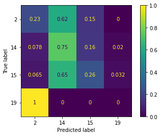
The confusion matrix allows us to compare the actual space group of the validation data, with that from the classification. For a perfect classification, you would have an identity matrix with the dimension of the number of labels.
Exercise
It is clear from the above confusion matrix, that our current selection of columns of interest is not sufficient to accurately classify the data. In this exercise, you should try different combinations of the columns of interest to see which give the best classification of the space group for these materials.