import matplotlib.pyplot as plt
from sklearn.datasets import make_blobs
from sklearn.ensemble import RandomForestClassifier
from dt_visualise import show, show_prob
Random forests
The idea that by combining multiple decision trees, all of which overfit, we can reduce the overfitting is an ensemble method known as bagging. Having multiple parallel estimators averaging gives a better classification. The specific application of this logic to decision trees is commonly known as a random forest.
The scitkit-learn module includes an optimised ensemble of random decision trees in the RandomForestClassifier estimator.
Let’s apply this to the data from the decision tree example.
X, y = make_blobs(n_samples=300, centers=4, random_state=0, cluster_std=1.0)
model = RandomForestClassifier(n_estimators=100)
fig, axes = plt.subplots(1, 1, figsize=(6, 4))
show(model, X, y, axes)
plt.show()
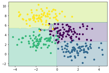
From the averaging of 100 random decision trees, we end up with an overall model that is much closer to our intuition about how the data should be segmented.
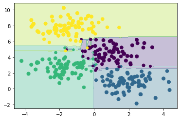
This offers a probabilistic classification of our data, due to the large number of decision trees utilised, in the show_prob plotting method, we scale the size of the dot based on the probability that the classification is correct.
Note that in area of uncertainty (near the middle) the dots are smaller than on the outside.
fig, axes = plt.subplots(1, 1, figsize=(6, 4))
show_prob(model, X, y, axes)
plt.show()
Let’s look now at a practical application of random forest classification in materials science.