import numpy as np
import matplotlib.pyplot as plt
from sklearn.decomposition import PCA
np.random.seed(1)
Principal Component Analysis
Principal component analysis (PCA) is a form of unsupervised machine learning method. We can understand PCA visually with a simple two-dimensional toy example. A deep discussion of the mathematical underpinnings of the PCA algorithm can be found in Bro and Smilde [BS14].
X = np.dot(np.random.rand(2, 2), np.random.randn(2, 200)).T
plt.plot(X[:, 0], X[:, 1], 'o')
plt.xlabel('x')
plt.ylabel('y')
plt.axis('equal')
plt.show()
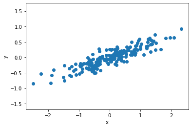
If we approach this data with linear regression, then we would obtain a model that describes the values of y that can be obtained from a given value of x.
However, in unsupervised learning, we aim to learn about the relationship between x and y-values.
PCA describes this relationship through a list of principal axes in the data.
The scikit-learn package includes a simple PCA estimator.
pca = PCA(n_components=2)
pca.fit(X)
PCA(n_components=2)
The fitting obtains information about the components and explained variance in the data.
print(pca.components_)
[[-0.94446029 -0.32862557]
 [-0.32862557  0.94446029]]
print(pca.explained_variance_)
[0.7625315 0.0184779]
We can visualise these as vectors over our data, where the components are the vector direction and the explained variance is the squared-length.
arrow = dict(arrowstyle='->', linewidth=2)

plt.plot(X[:, 0], X[:, 1], 'o', alpha=0.2)
for length, vector in zip(pca.explained_variance_, pca.components_):
    v = vector * 3 * np.sqrt(length)
    plt.annotate('', pca.mean_ + v, pca.mean_, arrowprops=arrow)
plt.axis('equal')
plt.show()
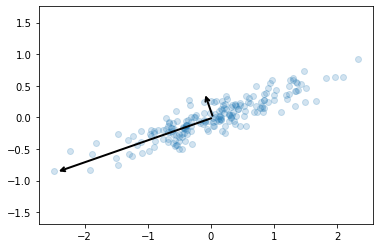
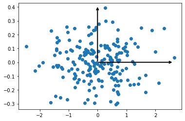
These vectors are the data’s principal axes and the length is an indication of the importance of the axis in describing the data (it is a measure of the variance when the data is projected onto that axis). We can plot the principal components, which is where each data point is projected onto the principal axes.
X_pca = pca.transform(X)
T_pca = PCA(n_components=2)
T_pca.fit(X_pca)

plt.plot(X_pca[:, 0], X_pca[:, 1], 'o')
for length, vector in zip(T_pca.explained_variance_, T_pca.components_):
    v = vector * 3 * np.sqrt(length)
    plt.annotate('', T_pca.mean_ + v, T_pca.mean_, arrowprops=arrow)
plt.show()
The PCA algorithm has some far-reaching real world applications, including assisting with data exploration and, as we will see later, in noise reduction.